Day 4: Spatial Data
Kathleen Hablutzel
7/9/2020
Getting Started
Here is the recording of today’s lesson. (This is only accessible within the NCSSM organization.) You can also follow along with the code below.
Today we will:
- Create static maps using
sfandggplot2 - Create interactive maps using
leaflet
You’ll need to install the sf and leaflet packages for later in the lesson. The sf package has multiple external dependencies, so pay close attention to any error messages during your install.
Notes Moving Forward
Schedule: Next week will be our last week of content. We will cover version control with GitHub and assorted R programming concepts, such as functions and iteration.
Resources: I am compiling a list of further R references and resources, as well as an FAQ from student questions throughout this course.
Guarantee: This website will stay on my GitHub as long as my GitHub exists, so this course will be available for years to come. I might slightly rearrange content so this website becomes a self-explanatory course, and I will convert the lessons to YouTube videos (with all student information removed) so the lectures will be available as well.
Last Week’s Challenges
Last week, I challenged you to find assorted information about the relational data in nycflights13 and fix a couple untidy data sets. The solutions are long enough that I have moved the solutions to the bottom of this page.
Spatial Data with sf
sf stands for simple features. Computers use features to represent real-world objects that have both spatial and non-spatial attributes. For example, North Carolina counties have geometries, such as county borders, and non-spatial attributes, such as names and populations.
Let’s load some spatial data. Unzip this shapefile of NC counties from the NC Department of Environmental Quality, and place the folder wherever you store your data for this course. Let’s read in the shapefiles using read_sf():
library(sf)
# load county shapefiles
counties <- read_sf("./data/NC_counties-shp")Note that I am loading the entire folder of files, not a particular file within the folder.
Let’s take a look at this data. We have exactly 100 counties, with lots of attributes such as CO_NAME and ACRES. The last column, geometry, always contains the spatial information for any spatial dataset.
View(counties)Thus, any spatial dataset will have two types of columns: a geometry column for the spatial data of a feature, and attribute columns for other information about each feature. In this dataset, the geometries are all POLYGON.
# what class is the geometry column?
counties %>%
pull(geometry) %>% # pulls the geometry column from the dataframe
class()## [1] "sfc_POLYGON" "sfc"See the simple feature documentation for more geometry types, including POINT and LINESTRING.
Static Maps with ggplot2
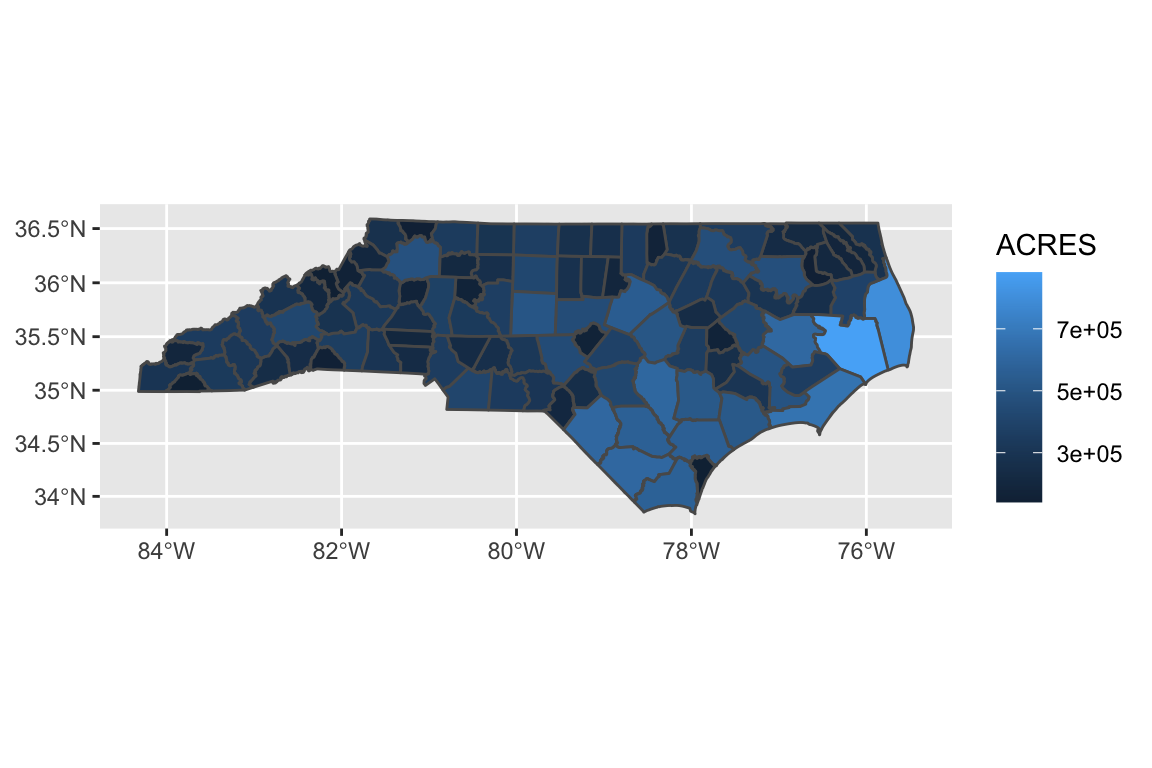
Let’s start exploring this spatial data. If we use the geom_sf() function, ggplot2 automatically knows to map x and y to the geometry column!
ggplot(data = counties, aes(fill = ACRES)) +
geom_sf()
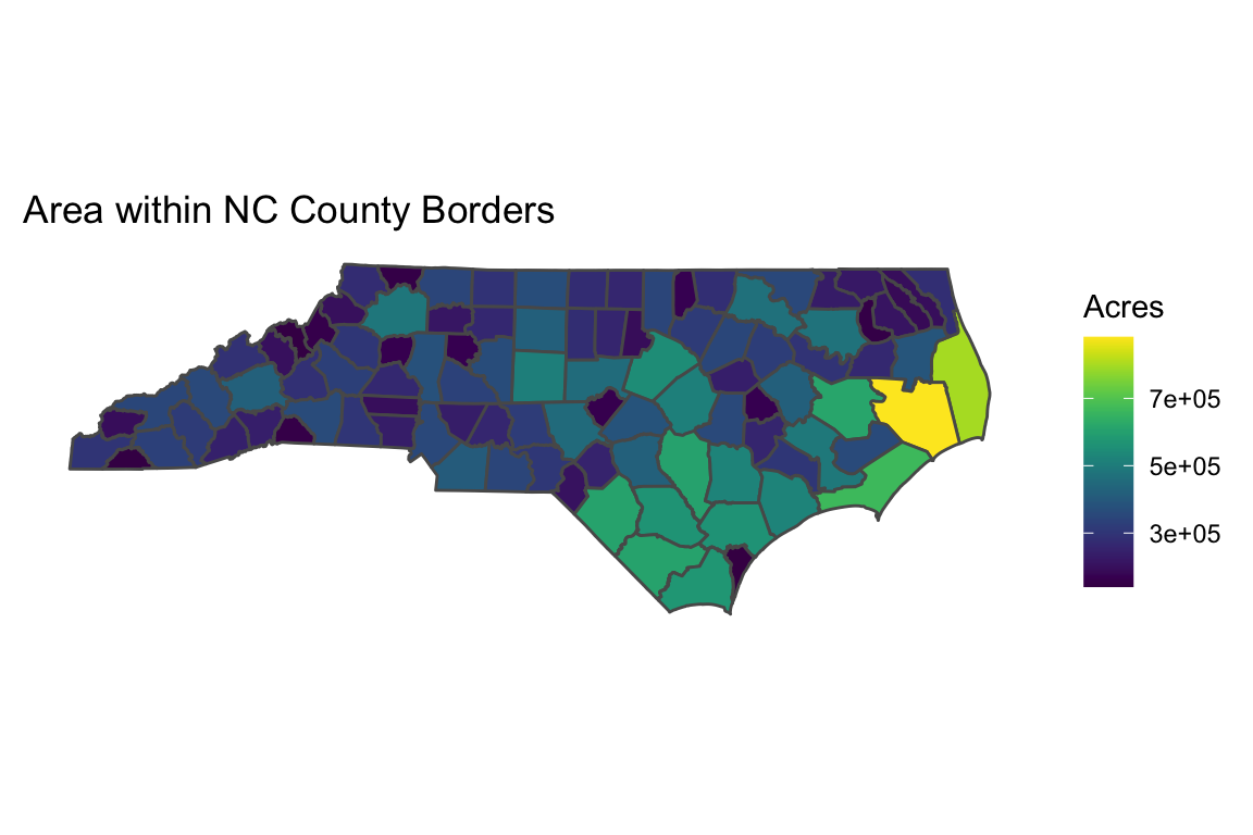
Then, we can alter our plot in the same way as any other ggplot.
library(viridis)
ggplot(data = counties, aes(fill = ACRES)) +
geom_sf() +
scale_fill_viridis() + # from the viridis package
labs(title = "Area within NC County Borders",
fill = "Acres") + # rename legend
theme(
rect = element_blank(), # remove background axes
axis.text = element_blank(), # remove axes
axis.ticks = element_blank()
)
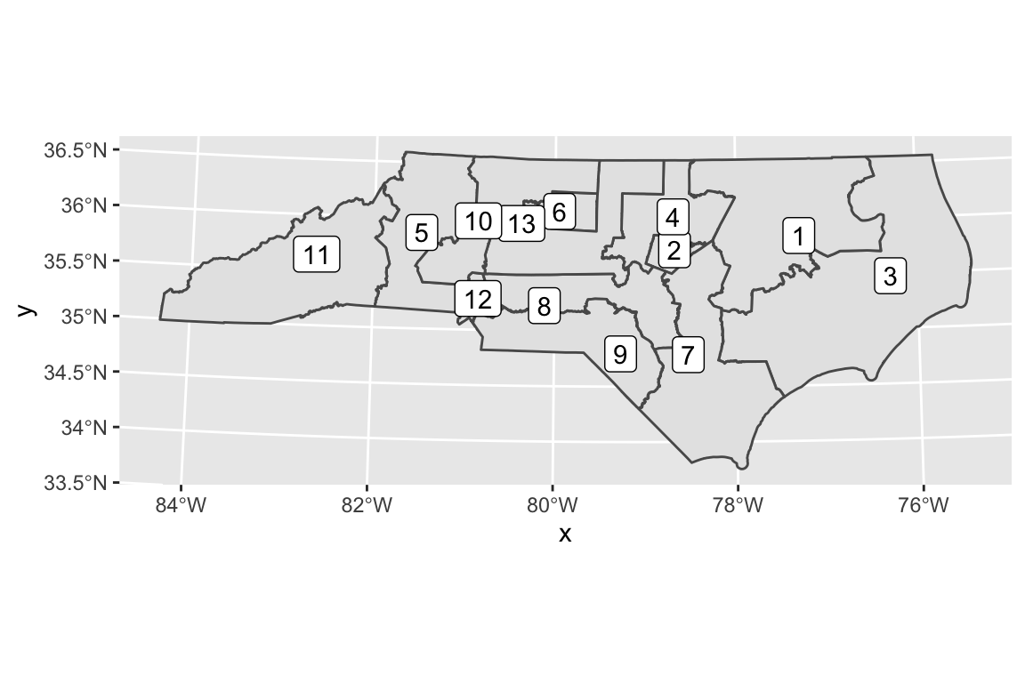
You can even layer multiple datasets of spatial features onto one map. Let’s download the NC Congressional District borders shapefile from the NC General Assembly redistricting website. Again, unzip the file and place it wherever you store your data.
nc_cd <- read_sf("./data/HB1029 3rd Edition - Shapefile")If you have trouble reading in the data, you might need to replace the spaces with a dash or underscore. (This is why spaces in filenames are bad practice!)
# just the congressional district data
ggplot(data = nc_cd) +
geom_sf() +
geom_sf_label(aes(label = DISTRICT)) # place labels in each district
When you overlay your shapefiles, make sure the map projections match. If not, you can transform one dataset to match another’s projection.
# county data projection
st_crs(counties) # number 3857: Pseudo-Mercator## Coordinate Reference System:
## User input: 3857
## wkt:
## PROJCS["WGS 84 / Pseudo-Mercator",
## GEOGCS["WGS 84",
## DATUM["WGS_1984",
## SPHEROID["WGS 84",6378137,298.257223563,
## AUTHORITY["EPSG","7030"]],
## AUTHORITY["EPSG","6326"]],
## PRIMEM["Greenwich",0,
## AUTHORITY["EPSG","8901"]],
## UNIT["degree",0.0174532925199433,
## AUTHORITY["EPSG","9122"]],
## AUTHORITY["EPSG","4326"]],
## PROJECTION["Mercator_1SP"],
## PARAMETER["central_meridian",0],
## PARAMETER["scale_factor",1],
## PARAMETER["false_easting",0],
## PARAMETER["false_northing",0],
## UNIT["metre",1,
## AUTHORITY["EPSG","9001"]],
## AXIS["X",EAST],
## AXIS["Y",NORTH],
## EXTENSION["PROJ4","+proj=merc +a=6378137 +b=6378137 +lat_ts=0.0 +lon_0=0.0 +x_0=0.0 +y_0=0 +k=1.0 +units=m +nadgrids=@null +wktext +no_defs"],
## AUTHORITY["EPSG","3857"]]# congressional district projection
st_crs(nc_cd) # 32119: NAD83 / North Carolina## Coordinate Reference System:
## User input: 32119
## wkt:
## PROJCS["NAD83 / North Carolina",
## GEOGCS["NAD83",
## DATUM["North_American_Datum_1983",
## SPHEROID["GRS 1980",6378137,298.257222101,
## AUTHORITY["EPSG","7019"]],
## TOWGS84[0,0,0,0,0,0,0],
## AUTHORITY["EPSG","6269"]],
## PRIMEM["Greenwich",0,
## AUTHORITY["EPSG","8901"]],
## UNIT["degree",0.0174532925199433,
## AUTHORITY["EPSG","9122"]],
## AUTHORITY["EPSG","4269"]],
## PROJECTION["Lambert_Conformal_Conic_2SP"],
## PARAMETER["standard_parallel_1",36.16666666666666],
## PARAMETER["standard_parallel_2",34.33333333333334],
## PARAMETER["latitude_of_origin",33.75],
## PARAMETER["central_meridian",-79],
## PARAMETER["false_easting",609601.22],
## PARAMETER["false_northing",0],
## UNIT["metre",1,
## AUTHORITY["EPSG","9001"]],
## AXIS["X",EAST],
## AXIS["Y",NORTH],
## AUTHORITY["EPSG","32119"]]# transform CDs to match counties
nc_cd <- nc_cd %>%
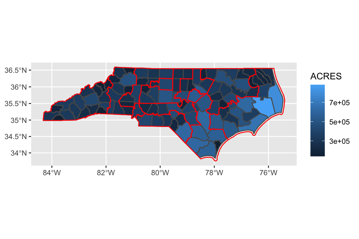
st_transform(3857)We transformed the Congressional Districts’ NAD83 / North Carolina projection into the counties’ Pseudo-Mercator projection. Now, we can overlay the maps successfully:
ggplot() +
geom_sf(data = counties, aes(fill = ACRES)) +
geom_sf(data = nc_cd,
fill = NA,
color = "red")
For most audiences, a static map is sufficient to display your spatial information. However, if you want to make something more interactive, you can use the leaflet package.
Interactive Maps with leaflet
Leaflet is an “open-source JavaScript library for mobile-friendly interactive maps.” The leaflet package for R integrates Leaflet with R.
Leaflet only works with data in the World Geodetic System 1984 projection, number 4326, so let’s transform our data:
counties_4326 <- counties %>%
st_transform(4326)
nc_cd_4326 <- nc_cd %>%
st_transform(4326)Our base leaflet map is just the map information:
library(leaflet)
leaflet() %>%
addTiles()Then, we use the pipe to add layers of information:
leaflet() %>%
addTiles() %>% # base map
addPolygons(data = counties_4326, # county outlines
color = "blue",
fillOpacity = 0.7) %>%
addPolygons(data = nc_cd_4326, # congressional district outlines
color = "red",
fillOpacity = 0,
label = ~DISTRICT) # hover over district to see numberlibrary(RColorBrewer)
pal <- colorNumeric(
palette = "Purples",
domain = counties_4326$ACRES)NC <- leaflet() %>%
addTiles() %>% # base map
addPolygons(data = counties_4326, # county outlines
color = ~pal(ACRES),
fillOpacity = 0.8) %>%
addPolygons(data = nc_cd_4326, # congressional district outlines
color = "red",
fillOpacity = 0,
popup = ~DISTRICT) # click on district to see numberncssm <- tribble(
~lat, ~lon, ~name,
36.018038, -78.920288, "Durham",
35.731852, -81.686701, "Morganton"
)NC %>%
addMarkers(data = ncssm,
popup = ~name)Computations with Spatial Data
Under construction (sorry)
returned vector, so add to data frame
See documentation for units
Spatial computations
nc_cd_4 <- nc_cd %>%
filter(DISTRICT == "4")
cd_4 <- counties %>%
filter(st_within(geometry, nc_cd, sparse = FALSE) |
st_intersects(geometry, nc_cd, sparse = FALSE))See cheatsheet
Challenges for Next Week
Let’s apply what we just learned! For next week, try to copy these maps: (coming soon)
As always, please Slack me throughout the week with any questions! I’ll reveal the code for these challenges next week.
Solutions For Last Week
Finally, here are the solutions to last week’s challenges:
# What is the average departure delay for each origin airport?
dep_delay <- flights %>%
group_by(origin) %>%
summarize(avg_dep_delay = mean(dep_delay, na.rm = TRUE))
# What is the average arrival delay for each destination airport?
arr_delay <- flights %>%
group_by(dest) %>%
summarize(avg_arr_delay = mean(arr_delay, na.rm = TRUE))
# Find all the flights that flew over 400 miles. What were their destinations?
# Version 1:
long_distance_A <- flights %>%
filter(distance > 400) %>%
group_by(dest) %>%
summarize() %>% # if we don't calculate new columns, we just have the unique destinations
left_join(airports, by = c("dest" = "faa")) %>% # to find names
select(dest, name)
# Version 2:
long_distance_B <- flights %>%
filter(distance > 400) %>%
select(dest) %>%
unique() %>% # removes duplicate entries
left_join(airports, by = c("dest" = "faa")) %>% # to find names
select(dest, name)
# Which airport was the most common destination? (What is its name?)
common_dest <- flights %>%
group_by(dest) %>%
summarize(num_flights = n()) %>%
arrange(desc(num_flights)) %>%
head(1) %>%
left_join(airports, by = c("dest" = "faa")) # find airport information
# Are there any planes in the `flights` table that don't appear in the `planes` table?
missing_planes <- flights %>%
filter(!is.na(tailnum)) %>% # remove flights with missing tail numbers
group_by(tailnum) %>%
summarize() %>% # unique tailnums
left_join(planes, by = c("tailnum" = "tailnum")) %>%
filter(is.na(type)) %>%
nrow() # count how many missing planes
# Among the 100 most commonly used planes, what is the most common manufacturer? Most common model?
# 100 most commonly used planes
common_planes <- flights %>%
filter(!is.na(tailnum)) %>% # remove flights with missing tail numbers
group_by(tailnum) %>%
summarize(num_flights = n()) %>%
arrange(desc(num_flights)) %>%
head(100)
# most common manufacturer
common_manufacturer <- common_planes %>%
left_join(planes, by = c("tailnum" = "tailnum")) %>% # get manufacturer data
group_by(manufacturer) %>%
summarize(num_made = n()) %>%
arrange(desc(num_made)) %>%
head(1)
# most common model
common_model <- common_planes %>%
left_join(planes, by = c("tailnum" = "tailnum")) %>% # get manufacturer data
group_by(model) %>%
summarize(num_flown = n()) %>%
arrange(desc(num_flown)) %>%
head(1)
# untidy data: lengths and albums of Bill Withers songs
untidyA <- tribble(
~artist, ~song, ~type, ~info,
"Bill Withers", "Ain't No Sunshine", "Length", "2:05",
"Bill Withers", "Ain't No Sunshine", "Album", "Just As I Am",
"Bill Withers", "Lovely Day", "Length", "4:15",
"Bill Withers", "Lovely Day", "Album", "Menagerie",
"Bill Withers", "Lean on Me", "Length", "4:19",
"Bill Withers", "Lean on Me", "Album", "Still Bill",
"Bill Withers", "Use Me", "Length", "3:48",
"Bill Withers", "Use Me", "Album", "Still Bill",
"Bill Withers", "Grandma's Hands", "Length", "2:01",
"Bill Withers", "Grandma's Hands", "Album", "Just As I Am"
)
# tidy version: pivot wider (There are multiple rows per observation/song.)
tidyA <- untidyA %>%
pivot_wider(names_from = "type", values_from = "info")
# untidy data: most popular songs on Spotify, for an eclectic mix of artists from Kathleen's playlists
untidyB <- tribble(
~artist, ~`1`, ~`2`, ~`3`, ~`4`, ~`5`,
"Bill Withers", "Ain't No Sunshine", "Lovely Day", "Lean on Me", "Use Me", "Grandma's Hands",
"Led Zeppelin", "Stairway to Heaven", "Immigrant Song", "Whole Lotta Love", "Black Dog", "Good Times Bad Times",
"The Supremes", "You Can't Hurry Love", "Baby Love", "Stop! In The Name Of Love", "Where Did Our Love Go", "Come See About Me",
"Alessia Cara", "Scars To Your Beautiful", "Out Of Love", "Stay", "Ready", "I Choose",
"Hozier", "Take Me To Church", "The Bones", "Almost", "Cherry Wine", "Like Real People Do"
)
# tidy version: pivot longer (The column names 1-5 are a variable, rank.)
tidyB <- untidyB %>%
pivot_longer(c(`1`, `2`, `3`, `4`, `5`), names_to = "rank", values_to = "title")