Day 3: Data Wrangling with dplyr

Getting Started

Here is the recording of today’s lesson. (This is only accessible within the NCSSM organization.) You can also follow along with the code below.

Today we will:

• Learn the 5 key verbs of dplyr
• Create pipelines with the pipe operator %>%
• Reorganize untidy data with tidyr
• Join data tables

You’ll need to install the nycflights13 package for later in the lesson.

Notes on Good Coding Practice

Comment your code: Use a # to leave comments in your code. Whether you call it a hash, hashtag, pound sign, number symbol, or octothorp, anything you write in your code after this useful symbol will not run. Comment to explain the purpose of key lines of code; it’ll help out anyone else reading your code, including yourself revisiting that code in 6 months. For example:

may_air <- airquality %>%
  filter(Month == 5) # only keep rows for May

Use readable, consistent formatting: Writing all your code on one line, crunching code together with no spaces, and naming objects x or y makes your code hard to read and interpret. Make your code readable, make your object names descriptive, and keep your formatting consistent. Take a look at this style guide for a readable example.

Source: https://xkcd.com/1513/

Last Week’s Challenges

Last week, I challenged you to copy two graphs. I don’t expect you to have gotten everything, but here’s the code:

star_plot <- ggplot(data = starwars, aes(x = height, y = mass)) + # starwars data
  geom_point(aes(color = gender)) + # scatterplot
  scale_color_brewer(palette = "Set1") + # colors
  labs( # various labels
    title = "Mass vs. Height of Star Wars Characters by Species",
    caption = "Source: Star Wars API", # at bottom
    x = "Height (cm)", # x-axis
    y = "Weight (kg)", # y-axis
    color = "Gender" # legend
  ) +
  theme( # plot theme
    text = element_text(family = "Arial"), # change font
    rect = element_blank(), # no background rectangle
    axis.line = element_line(color = "gray40"), # axis line dark
    panel.grid = element_line(color = "gray90"), # grids light
    legend.position = "bottom" # legend at bottom
  )

star_plot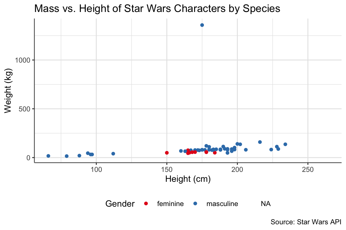

height_plot <- ggplot(data = starwars, aes(y = homeworld)) +
  geom_bar(fill = "#4F5810") + # bar chart (green bars)
  theme_solarized() +
  labs(
    title = "Number of Starwars Characters by Homeworld",
    subtitle = "As recorded in the starwars dplyr dataset", # subtitles are possible too!
    caption = "Source: Star Wars API",
    x = "Number of Characters",
    y = "Homeworld"
  )

height_plot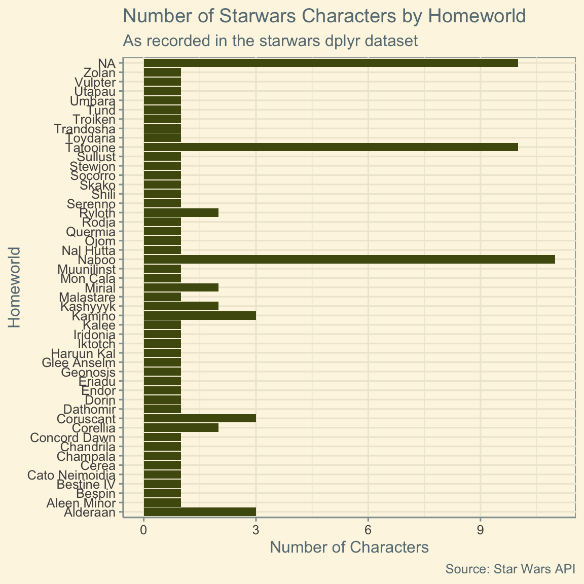

My default figure height and width are 4 and 6 respectively, but on the second graph, I set fig.height = 6.

Introduction to dplyr

The dplyr package provides a grammar for data transformation, just like how ggplot2 provides a grammar for graphics. In dplyr, various functions are verbs that specify actions to take on your data table.

For example,

starwars %>%
  arrange(height)

arranges the characters in the starwars dataset from shortest to tallest. The action is arrange(), and the object of the action is the starwars dataset.

Check out the dplyr documentation here for more information.

The Pipe Operator

Source: magrittr package

When we want to apply multiple functions in a row to our data, what are our options?

We can work one function at a time, feeding each resulting dataframe into our next verb. For example, to tell little bunny foo-foo to hop, then scoop, then bop:

result1 <- hop(foo_foo, through = "forest")

result2 <- scoop(result2, up = "field_mice")

result3 <- bop(result3, on = "head")

This seems inefficient. Can we do this all at once?

result3 <- bop(scoop(hop(foo_foo, through = "forest"), up = "field_mice"), on = "head")

This nested form is really hard to read, especially when we add more and more verbs, each with multiple arguments.

This is why we use the pipe. The pipe operator uses the result of the previous line as the dataset for the next function. We end up with a list of actions to take, all in order:

result3 <- foo_foo %>%
  hop(through = "forest") %>%
  scoop(up = "field_mice") %>%
  bop(on = "head")

We know to take the data foo_foo and apply the functions hop(), scoop(), and bop() in that order, using the result of one line as the data for the next.

Read more about the pipe operator here.

The Five Verbs of dplyr

Now, let’s finally discuss these five verbs of dplyr!

arrange()

Sort the rows of a dataset based on some column:

starwars %>%
  arrange(height)

This sorts the Star Wars characters from shortest to tallest.

Alternately, to sort highest to lowest values, add desc():

starwars %>%
  arrange(desc(height))

This sorts the Star Wars characters from tallest to shortest.

Note: We can also use the head() function to get the first N rows of a dataframe. If we want the 10 tallest starwars characters, we could write:

starwars %>%
  arrange(desc(height)) %>%
  head(10)

mutate()

Add or modify a column. Calculate the new column entries based on some formula or criteria.

# add new column height_ft
starwars %>%
  mutate(height_ft = height / 30.48) 

# replace height column with heights in ft, not cm
starwars %>%
  mutate(height = height / 30.48)

Note: we didn’t store the result, so we didn’t actually change starwars

# add new column for whether character is taller than 80 cm
starwars %>%
  mutate(height = height >= 80)

# add new column for character BMI
starwars %>%
  mutate(bmi = mass / (height ** 2) / 100)

select()

Select which columns of a dataset to keep.

# only keep the name, height, and mass columns
starwars %>%
  select(name, height, mass)

Alternately, specify which columns to drop. Note the minus sign (-) before the column names.

# keep all columns EXCEPT name, height, and mass
starwars %>%
  select(-name, -height, -mass)

filter()

Keep the rows that meet certain conditions.

# height above 80 cm
starwars %>%
  filter(height >= 80)

# species: Hutt
starwars %>%
  filter(species == "Hutt")

# species: Hutt or Wookiee
starwars %>%
  filter(species %in% c("Hutt", "Wookiee"))

# multiple criteria
starwars %>%
  filter(height > 80, # and
         mass > 40)

starwars %>%
  filter(height > 80 & mass > 40) # and

starwars %>%
  filter(height > 80 | mass > 40) # or

To make a list (a vector) of multiple values, surround them with c(). Then, we can filter for species %in% the vector.

Multiple conditions can be separated with commas to look for rows with criteria1 AND criteria2. Alternately, conditions can be written as criteria1 & criteria2 (and) or criteria1 | criteria2 (or). The “or” condition uses the vertical bar towards the top right of your keyboard.

summarize()

Create a new table that shows a summary of the data.

# count number of rows
starwars %>%
  summarize(num_rows = n()) # n() is a function that counts rows

# number of rows, average height, average mass, and min birth year
starwars %>%
  summarize(num_rows = n(),
            avg_height = mean(height),
            avg_mass = mean(mass, na.rm = TRUE),
            min_birth = min(birth_year, na.rm = TRUE))

Note that in the mean() and min() summary functions, we have to specify na.rm = TRUE to ignore the NA values in our data. Otherwise, the result is NA. Other useful summary functions are listed in the summarise() documentation here. (The summarize() function can also be called summarise() with an s.)

So far, summarize() only returns one row, with summaries for the data set as a whole. What if we want to summarize for different groups, such as finding the average height for each species?

We often pair summarize() with the function group_by(). This function converts a table into a grouped table, where operations are performed “by group.”

starwars %>%
  group_by(species) %>%
  summarize(N = n(),
            avg_height = mean(height, na.rm = TRUE),
            avg_mass = mean(mass, na.rm = TRUE),
            min_birth = min(birth_year, na.rm = TRUE))

Now, we have the counts, averages, and minimums for each species: the average human mass, the average Wookiee mass, etc. Note that the new dataframe maintains our group columns as well as the columns we specify within summarize().

Combining Verbs

Often, we need to combine multiple verbs to get the result we need. We can list each verb in order using pipes. For example, if we want to find the 5 most common species of female characters, our pipeline would look like this:

f_common_species <- starwars %>%
  filter(gender == "female") %>% # only female characters
  group_by(species) %>%
  summarize(N = n()) %>% # count characters for each species
  arrange(desc(N)) %>%
  head(5)

f_common_species

In the result, one of the species is NA. dplyr grouped together all the characters with unknown species. To remove these characters, we could add another criterium to our filter() function: !is.na(species). The is.na() function checks whether the species is NA, and the ! means “not”, so together our criteria are for species to be “not NA.”

f_common_species <- starwars %>%
  filter(gender == "female", # only female characters
         !is.na(species)) %>% # exclude characters with unknown species
  group_by(species) %>%
  summarize(N = n()) %>% # count characters for each species
  arrange(desc(N)) %>%
  head(5)

f_common_species

For more information on these 5 verbs of dplyr, check out the dplyr cheatsheet and data wrangling cheatsheet. These cheatsheets also visualize each function, so I recommend taking a look.

Tidy Data

Let’s pivot topics now to discuss organizing data. The easiest type of data to use in the tidyverse is tidy data, where each variable has its own column, each observation has its own row, and each value has its own cell. This simple and consistent format works most naturally within the tidyverse.

Unfortunately, much of the data you encounter will be untidy. How do we tidy up our data? We use the tidyr package. If one variable is spread across multiple columns, we use pivot_longer(), and if one observation is scattered across multiple rows, we use pivot_wider().

pivot_longer()

We use pivot_longer() when one variable is spread across multiple columns. For example, the following table of country populations uses multiple columns for the year variable:

untidy_wide <- tribble(
  ~country, ~`2018`, ~`2019`,
  "USA", 306.8, 328.2,
  "Mexico", 126.2, 127.6,
  "Canada", 37.06, 37.59
)

untidy_wide

With pivot_longer(), we make the years one column and the populations a different column.

tidy_longer <- untidy_wide %>%
  pivot_longer(c(`2018`, `2019`), names_to = "year", values_to = "population")

tidy_longer

Our first argument is a vector specifying which column names to put in the new column: 2018 and 2019. We name this column of column names with names_to, and we name the column for the current values with values_to. Note: The column names are surrounded in backticks ` because they don’t follow standard column naming conventions (no spaces, and don’t start with a number).

I don’t expect this to be simple the first time, so play around with examples and check out this R for Data Science resource.

Here’s an example visualization for slightly different data:

From R for Data Science

pivot_wider()

pivot_wider() does the opposite of pivot_longer(). We use pivot_wider() when one observation is scattered across multiple rows. For example, the following table uses multiple rows to split up one observation, a country in a year. There’s one row for population (in millions), and then another row for number of births (per 1000 people).

untidy_long <- tribble(
  ~country, ~year, ~type, ~count,
  "USA", 2018, "population", 306.8,
  "USA", 2018, "births", 11.968,
  "USA", 2019, "population", 328.2,
  "USA", 2019, "births", 11.979,
  "Mexico", 2018, "population", 126.2,
  "Mexico", 2018, "births", 17.736,
  "Mexico", 2019, "population", 127.6,
  "Mexico", 2019, "births", 17.455,
  "Canada", 2018, "population", 37.06, 
  "Canada", 2018, "births", 10.376, 
  "Canada", 2019, "population", 37.59,
  "Canada", 2019, "births", 10.452
)

untidy_long

With pivot_wider(), we condense the observations into one row, with new columns for each type of value (in this case, a population column and a births column).

tidy_wider <- untidy_long %>%
  pivot_wider(names_from = "type", values_from = "count")

tidy_wider

We specify which column has the column names/types of values (names_from = "type") and which column has the values (values_from = "count").

Here’s an example visualization for slightly different data:

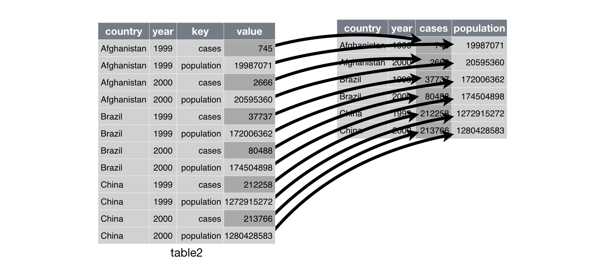
Again, I don’t expect this to be simple the first time, so play around with examples and check out this R for Data Science resource. Note that the data wrangling cheatsheet is outdated, so pivot_longer() is called gather() and pivot_wider() is called spread().

Joining Tables

Sometimes, we can also organize data across multiple tables. We call this relational data, and this organization is useful for large databases where we don’t always need the information from every table.

For example, the nycflights13 package provides multiple tables of different information on all 336,776 flights that departed from New York City’s three airports in 2013. The flights table lists all the flights, airlines has information on different carriers, airports lists information about different airports, etc. If I want to know the time zones of the airports where the flights ended up, I would have to match up the data from two different tables: flights and airports. As long as at least one column matches in both datasets, I can join the tables together:

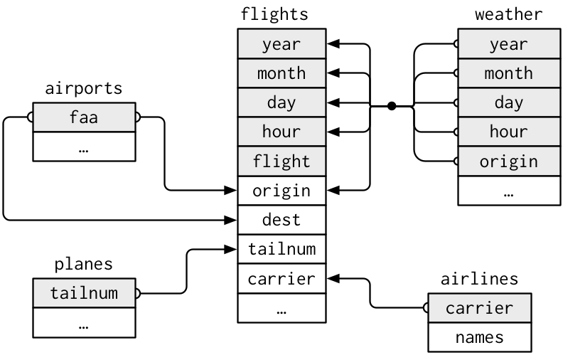
We can join flights with airports by matching flight destinations (in flights) with airport faa codes (in airports). We’ll get one big dataset that has all the airport information for each flight’s destination.

library(nycflights13)

flights %>%
  inner_join(airports, by = c("dest" = "faa"))

We pipe the first table into the function, write the second table as an argument, and then specify the by argument as a vector of corresponding column names, so the join function knows which columns to match up.

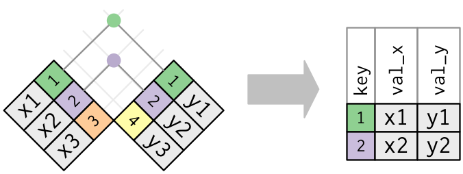
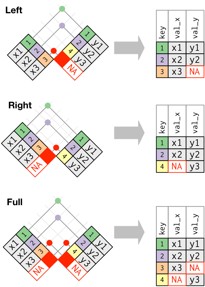
Let’s see different ways to join these tables together:

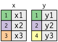
Inner Joins

• inner_join(): Only keep rows that match in both tables.

Outer Joins

• left_join(): Keep every row in the left table, even if there’s no match on the right. Some rows on the right get duplicated or excluded.

• right_join(): Keep every row in the right table, even if there’s no match on the left. Some rows on the left get duplicated or excluded.

• full_join(): Keep every row in both tables, regardless of whether there’s a match in the other table.

We can also picture these joins with a Venn Diagram:

These are all valid ways to join tables, and they all produce different results. Which join you use all depends on the context of your problem. (Note: We rarely use right joins, because a right join could get rearranged into a left join.)

flights %>%
  inner_join(airports, by = c("dest" = "faa"))

flights %>%
  left_join(airports, by = c("dest" = "faa"))

flights %>%
  right_join(airports, by = c("dest" = "faa"))

flights %>%
  full_join(airports, by = c("dest" = "faa"))

This is just a brief overview, so for more information on joins, head to R for Data Science, from where I’ve sourced all of today’s diagrams.

Challenges for Next Week

Let’s apply what we just learned! For next week, try to find:

• What is the average departure delay for each origin airport?
• What is the average arrival delay for each destination airport?
• Find all the flights that flew over 400 miles. What were their destinations?
• Which airport was the most common destination? (What is its name?)
• Are there any planes in the flights table that don’t appear in the planes table?
• Among the 100 most commonly used planes, what is the most common manufacturer? Most common model?

Also, how would I fix these untidy datasets?

Lengths and albums of Bill Withers songs:

untidyA <- tribble(
  ~artist, ~song, ~type, ~info,
  "Bill Withers", "Ain't No Sunshine", "Length", "2:05",
  "Bill Withers", "Ain't No Sunshine", "Album", "Just As I Am",
  "Bill Withers", "Lovely Day", "Length", "4:15",
  "Bill Withers", "Lovely Day", "Album", "Menagerie",
  "Bill Withers", "Lean on Me", "Length", "4:19",
  "Bill Withers", "Lean on Me", "Album", "Still Bill",
  "Bill Withers", "Use Me", "Length", "3:48",
  "Bill Withers", "Use Me", "Album", "Still Bill",
  "Bill Withers", "Grandma's Hands", "Length", "2:01",
  "Bill Withers", "Grandma's Hands", "Album", "Just As I Am"
)

untidyA

Most popular songs on Spotify, for an eclectic mix of artists from Kathleen’s playlists:

untidyB <- tribble(
  ~artist, ~`1`, ~`2`, ~`3`, ~`4`, ~`5`,
  "Bill Withers", "Ain't No Sunshine", "Lovely Day", "Lean on Me", "Use Me", "Grandma's Hands",
  "Led Zeppelin", "Stairway to Heaven", "Immigrant Song", "Whole Lotta Love", "Black Dog", "Good Times Bad Times",
  "The Supremes", "You Can't Hurry Love", "Baby Love", "Stop! In The Name Of Love", "Where Did Our Love Go", "Come See About Me",
  "Alessia Cara", "Scars To Your Beautiful", "Out Of Love", "Stay", "Ready", "I Choose",
  "Hozier", "Take Me To Church", "The Bones", "Almost", "Cherry Wine", "Like Real People Do"
)

untidyB

Finally, if you’re curious, you can check out Hadley Wickham’s paper on Tidy Data.

As always, please Slack me throughout the week with any questions! I’ll reveal the code for these challenges next week.

---

See the GitHub repo, or contact me via my personal website.

Credit: Course and website by Kathleen Hablutzel, NCSSM '19, Smith College SDS+CS '23.

Almost everything I share, I learned from Smith College's SDS 192 Introduction to Data Science course by Ben Baumer and R. Jordan Crouser.